

In practise, Guass's law is used in either one of two ways: if I tell you the distribution of charges \(q_{enc}\) in a region of space, then you can use Guass's law to determine the electric field \(\vec{E}\) produced by that charge distribution at each point along a closed, imaginary surface; and vice versa, if I tell you what the electric field \(\vec{E}\) is at each point along a closed surface, then you can use Guass's law to determine the distribution of charges \(q_{enc}\) inside of that surface. That's how we use Guass's law to solve problems, in a nutshell. Let's begin by looking at a very simple example of finding \(\vec{E}\) along each point on a closed surface given that we know what \(q_{enc}\) is: we'll use Guass's law to find the electric field \(\vec{E}\) produced by a single point charge \(q\). We already know from experiments and, also, using Column's law and mathematics, that the electric field produced by a point charge is given by \(\vec{E}=k\frac{q}{r^2}\hat{r}\). But let's show that Guass's law predicts this same correct result.
Recall that in the previous lesson, we were able to use Column's law (plus a lot of math) to derive Guass's law which is given by
$$∮\vec{E}·d\vec{A}=\frac{q_{etc}}{Ɛ_0},tag{1}$$
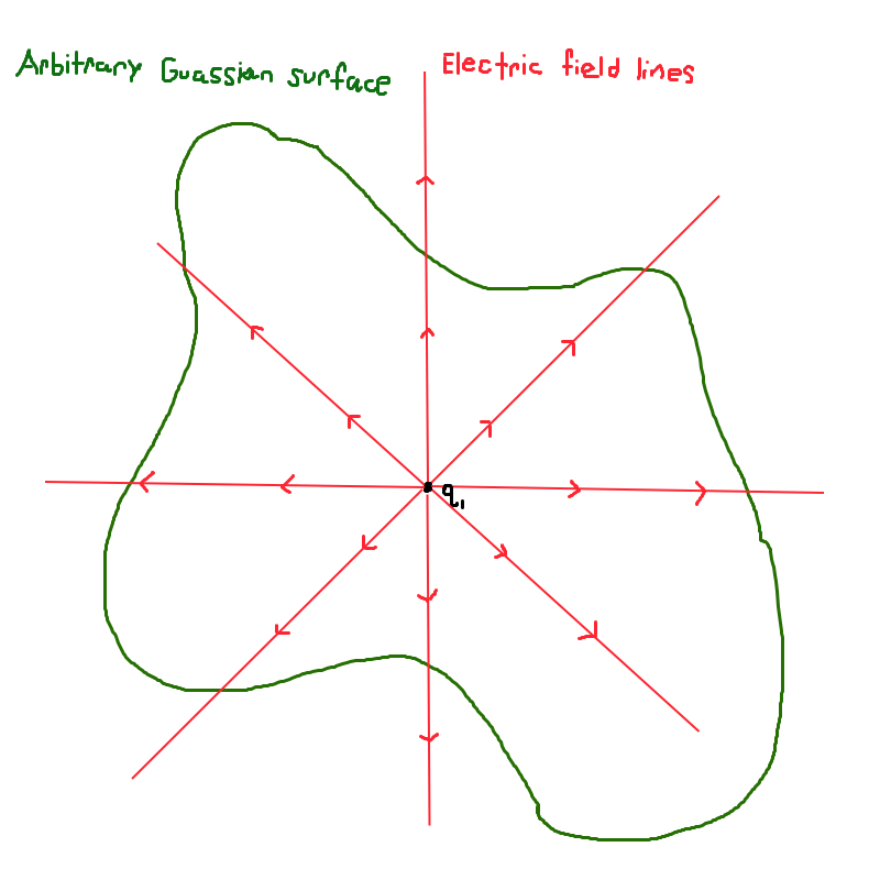
Figure 1
where \(\vec{E}\) is the electric field vector at each point along any arbitrary surface, \(d\vec{A}\) is also a vector at each point along that surface, and \(q_{enc}\) is just the total charge on the "inside" of that surface. We're trying to find the electric field produced by a single point charge; but the problem is that the integral in Equation (1) is very messy. A general principle (which we'll use in this problem and next several problems) which is used in many problems whenever we're trying to use Guass's law to find \(\vec{E}\) given \(q_{enc}\) is this: we want to simplify that integral in Equation (1) so we can easily (using just some algebra) find \(\vec{E}\) by choosing a surface which simplifies the integral \(\int\vec{E}.d\vec{A}\) to just \(E∮dA=E(\text{surface area})\). Let's see how this simplification would apply to our point charge example. Let's choose our arbitrary closed surface enclosing \(q\) to be a sphere. Will this choice of surface simplify the integral in the way that we want? In Figure 1, I have drawn th field lines of a \(q\) to show, qualitatively, that the direction of \(\vec{E}\) is always pointing radially outward. (The field lines of a single point charge can be experimentally determined as shown in Figure 2.) In this problem (and in the next several problems), step one to simplifing the integral \(∮\vec{E}·d\vec{A}\) is to simplify \(\vec{E}·d\vec{A}\) to \(EdA\) by choosing the right surface. Does this simplification occur when we choose a sphere? Recall from the previous lessons (and, in particular, the lesson on electric flux) that \(\vec{E}·d\vec{A}\) is a collection of infintelly many terms in the infinite sum, \(∮\); each term, \(\vec{E}·d\vec{A}\), is evaluated on each point along the surface. Also recall that the vector \(d\vec{A}\) is, by definition, normal (and perpendicular) to the surface at each point and is, also, by convention, always pointing in the "outward" direction - that is, away from the inside of the surface. If we translate that statement in to a picture, the vector field \(d\vec{A}\) looks like that shown in Figure 2. Given the field lines produced by \(q\) (which can be deduced from experiments like that shown in Figure 2), we also know that \(\vec{E}\) is always pointng in the radial outwar direction at every point. This means that the vector fields \(\vec{E}\) and \(d\vec{A}\) must be parallel and pointing in the same direction to each other at every point along the surface. Thus, from the definition of the dot product, every term \(\vec{E}·d\vec{A}\) in the infinite sum, \(∮\), simplifies to \(\vec{E}·d\vec{A}=EdAcos0=EdA\). Thus, we can simplify Equation (1) to
$$∮EdA=\frac{q_{enc}}{\epsilon_0}.\tag{2}$$

Figure 2

Figure 3
Notice that if we just choosed any whacky surface, this simplification would, in general, not have occured. For example, suppose that we chose the surface illustrated in Figure 3. \(\vec{E}\) has to always point in the radial outward direction; but \(d\vec{A}\) has to always be normal to the surface. This is why \(\vec{E}\) and \(d\vec{A}\) are not parrellel and at an angle \(\theta\) to one another at many of the points along the surface. If we chose this surface, then we could not have made our simplification and \(\vec{E}·d\vec{A}≠EdA\).
The second and final step to simplifying our integral is to make sure that we not only chose a surface for which \(\vec{E}·d\vec{A}≠EdA\), but also a surface where the magnitude of the electric field \(E\) at each point is constant allowing us to further simplify the integral to \(∮EdA=E∮dA\). The field lines of \(q\) tell us not only qualitative information about the direction of \(\vec{E}\), but they also tell us qualitative information about the magnitude of \(E\) because the number of field lines \(N\) passing through a region of area \(A\) is proportional to \(E\) in that region. Since the same number of field lines pass through any arbitrary region along the surface, it follows that \(E\) is the same along each region of the sphere. Since \(E\) is constant everywhere alon the surface of the sphere, we can simplify Equation (2) to
$$∮E·dA=E∮dA=\frac{q_{enc}}{\epsilon_0}.\tag{3}$$
As I briefly mentioned earlier, once we have chosen a surface for which \(∮\vec{E}·d\vec{A}=E ∮ dA\), finding \(E\) just simplifies to a basic algebra problem. (Well, ignoring that finding \( ∮dA\) is technically calculus—but you'll see what I mean.) If we take the infinite sum, \(∮\), of the area of every surface element comprising any arbitrary surace (such as the sphere), we'll get the total surface area of that surface and \(∮dA=\text{surface area}\). (If you imagine each contribution of \(dA\) shading the surface as in Figure 2, you can see visually that each little \(dA\) will eventually add up to the area of the entire surface.) Thus, Equation (3) simplifies to
$$E∮dA=E(\text{surface area})=\frac{q_{enc}}{ɛ_0)}.\tag{4}$$
Let's divide Equation (4) by the surface area on both sides to isolate \(E\):
$$E=\frac{q_{enc}}{\epsilon_0(\text{surface area})}.\tag{5}$$
Since the surface area of a sphere is given by \(4 π r^2\) and since \(\epsilon_0=\frac{1}{4πk}\), Equation (5) simplifies to
$$E=\frac{4πkq}{4πr^2}=k\frac{q}{r^2}.\tag{6}$$
Thus, we have proven (at least for a point charge) that Guass's law makes the same prediction as Column's law (which is important since that is the result which agrees with experiement). From the field lines of \(q\), we can conclude that
$$\vec{E}=k\frac{q}{r^2}\hat{r}.\tag{7}$$
It is important to recall from the previous lesson that the electric field \(\vec{E}\) in Equation (1) is merely the electric field produced at every point along our chosen surface. You might think that we may therefore have solved for the electric field at each point along an imaginary sphere and not at every point in space. But we chose our surface to be any sphere of radius r. You can imagine redoing this problem for infinitely many different spheres each with a different radius \(r\) - you'll always go through all the same arguments and just end up getting \(E=k\frac{q}{r^2}\) every time.