Line integrals are used to find the area between a surface \(f(x,y)\) and any arbitrary curve. In this lesson, we'll define the idea of line integral and derive a formula for calculating them.

In this video, we’ll discuss Shkadov thrusters: a method of moving stars, star systems, and even entire galaxies.
The lack of oxygen in Mars' atmosphere and running liquid water on its surface is very inconveniant for any humans living their since oxygen and liquid water are necessary for humans to survive. Fortunatelly, there is an abundance of frozen water on Mars' surface. In this lesson, we'll discuss various techniques which can be used to extract all of this water. Once the water is obtained, by performing electrolysis on the water we can distill all of the oxygen from that water we need.
Line integrals are used to find the area between a surface \(f(x,y)\) and any arbitrary curve. In this lesson, we'll define the idea of line integral and derive a formula for calculating them.
In this lesson, we'll derive Maclaurin/Taylor polynomials which are used to "approximate" arbitrary functions which are smooth and continuous. More generally, they are used to give a local approximation of such functions. We'll also derive Maclaurin/Taylor series where the approximation becomes exact.
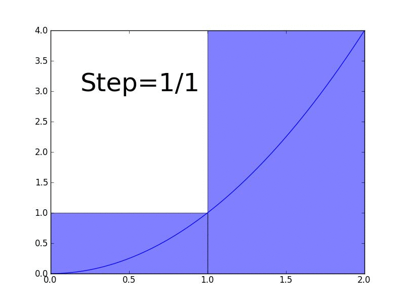
In this lesson, we define an integral as the Riemann sum as the number of rectangles approaches infinity.
A spaceship using an Alcubierre warp drive would involve assembling a ring of negative energy around the spaceship which would distort spacetime in this particular way: the spaceship sits in a "bubble" of flat, Minkowski spacetime which is "pushed" by expanding space behind it and "pulled" by contracting space infront of it. The spaceship does not move through space, but rather space itself moves and carries along the spaceship for the ride. Since general relativity places no limit on how fast space can move, the space can "carry" the warp bubble and spaceship away at faster than light (FTL) speeds.
Terraforming a world just means to make it more Earth-like. In this article, we'll discuss various techniques which have been proposed by scientists and engineers that would make Mars more like our home planet. We shall also discuss a potential scheme of future events which might occur as humans terraform and colonize Mars.
When Einstein was first working on developing his special theory of relativity, he was studying both Newtonian mechanics and Maxwell's equations: the two pillars of modern physics of his time. He noticed that these two theories contradicted one another in a very deep way. One of these pillars must fall. Newtonian mechanics implies the Galilean transformation equations—something which we are all already familiar with. These equations are consonant with our everyday intuitions: they tell us that velocities add. This makes sense: If I watch someone standing on top of semi throw a baseball at 5 m/s (in the same direction the truck is moving) and the truck wizzes by me at 30 m/s, then I'll see the baseball travel away from me at 35 m/s. But Maxwell's equations predict something very strange. These equations predict that a light beam will move away from you at the same speed whether your standing still or, as in another one of Einstein's thought experiments, "chasing" the light beam at 99% the speed of light. The reconciliation between Newtonian mechanics and Maxwell's equations is called the special theory of relativity. When we modify Newtonian mechanics to allow for the constancy of light speed for all observers, we get some very strange, bizarre, but also very profound consequences.
Time dilation is one of the many bizarre consequences of the speed of light being the same for everybody. For any observers in inertial frames of reference moving away from one another at a relative velocity which is close to that of the speed of light, they will see each others clocks run more slowly. In this section, we'll explore one of Einstein's original thought experiment: a train with a light clock moving past an observer standing idly at the train station. We'll see that the constancy of light speed with respect to all observers implies that time must slow down when watching events unfold in one frame of reference from another frame of reference if those two frames of reference are moving relative to each other. We'll start off by showing this for light beams bouncing off of two mirrors, but at the end we'll realize that this same argument applies to photons emitted between two atoms. The latter results in all physical clocks, chemical or biological, running more slowly.
In this section, we'll begin by seeing how Schrodinger's time-independent equation can be used to determine the wave function of a free particle. After that, we'll use Schrodinger's time-independent equation to solve for the allowed, quantized wave functions and allowed, energy eigenvalues of a "particle in a box"; this will be useful later on as a qualitative understanding of the quantized wave functions and energy eigenvalues of atoms.
Li-Fi was invented in 2011 by professor Harald Haas and is a form of wireless communications technology which would allow us to transmit information and data at least 100 times faster than Wi-Fi. Even more significantly, Li-Fi is essential—and in fact, it is necessary—for us to transition to a Third Industrial Revolution (TIR) infrastructure where everything in the environment—from buildings, roads, and walkways—becomes "cognified."
In this lesson, we'll use the concept of a definite integral to calculate the volume of a sphere. First, we'll find the volume of a hemisphere by taking the infinite sum of infinitesimally skinny cylinders enclosed inside of the hemisphere. Then we'll multiply our answer by two and we'll be done.
In this lesson, we'll give a friendly introduction to what nuclear fusion is and how it might be used by space faring civilizations.
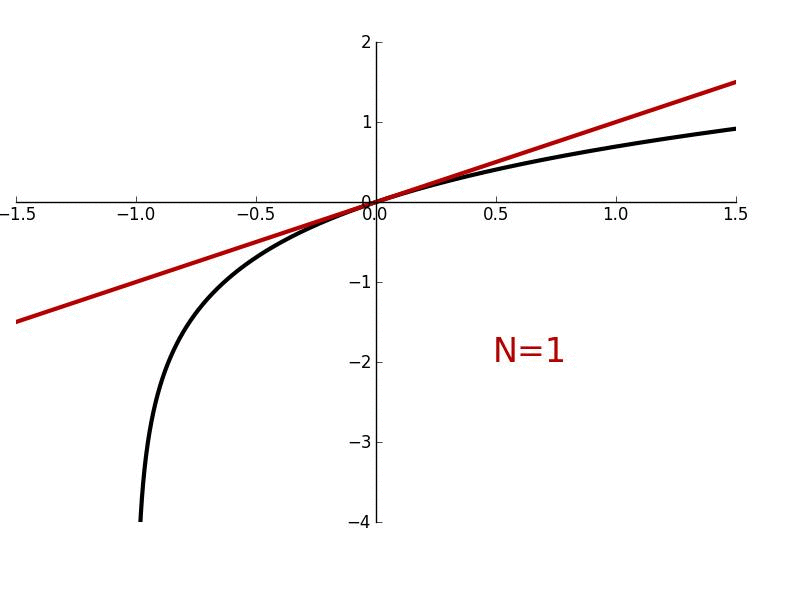
In this lesson, we'll find the integral of any arbitrary function \(kx^n\) where \(k\) and \(n\) are any finite numbers such that \(n≠-1\).
Capacitance is defined as the amount of charge stored in a capacitor per volt across the capacitor. The value of the capacitance is a measure of how rapidly a capacitor stores electric potential energy as the capacitor is getting charged up.
In this lesson, we'll determine the electric potential difference (also called voltage) across any arbitrary capacitor.
Complex numbers

Any ket vector \(|\psi⟩\) can be multiplied by a number \(z\) (which, in general can be real or complex) to produce a new vector \(|\phi⟩\):
$$z|\psi⟩=|\phi⟩.$$
In general, \(z=x+iy\). Sometimes the number \(z\) will just be a real number with no imaginary part, but in general it can have both a real and imaginary part. The complex conjugate of the number \(z\) is represented by \(z^*\) and is obtained by changing the sign of the imaginary part of \(z\); so \(z^*=x-iy\). Let’s look at some examples of complex numbers and their complex conjugates. Suppose that \(z\) is any real number with no imaginary part: \(z=x+(i·0)=x\). The complex conjugate of any real number is \(z^*=x-(i·0)=x\). In other words taking the complex conjugate \(z^*\) of any real number \(z=x\) just gives the real number back. Suppose, however, that \(z=x+iy\) is any complex number and we take the complex conjugate twice. Let’s see what we get. \(z^*\) is just \(z^*=x-iy\) (a new complex number). If we take the “complex conjugate of the complex conjugate,” we have \((z^*)^*=x+iy=z\). For any complex number \(z\),\(z^*=z\) .
If we multiply any complex number \(z\) by its complex conjugate \(z^*\), we’ll get
$$zz^*=(x=iy)(x-iy)=x^2-ixy+ixy-i^2y^2=x^2+y^2.$$

Figure 1: Any complex number \(z\) can be represented in either Cartesian coordinates as \(x+iy\) or in polar coordinates as \(re^{iθ}\).
For any complex number \(z\) the product \(z^*z\) is always a real number that is greater than or equal to zero. This product is called the modulus squared and, in a very rough sense, represents the length squared of a vector in a complex space. We can write the modulus squared as \(|z|^2=zz^*\). From Figure 1 we can also see that any complex number can be represented by \(z=x+iy=rcosθ+irsinθ=re^{iθ}\). The complex conjugate of this is \(z^*=x-iy=rcosθ+irsin(-θ)=re^{-iθ}\). The modulus squared of any vector in the complex plain is given by \(|z|^2=zz^*=(re^{iθ})(re^{iθ}=r^2\). If \(|z|^2=r^2=1\) and hence \(|z|=r=1\), then the magnitude of the complex vector is 1 and the vector is called normalized.
Column and row vectors and matrices
Any vector \(|A⟩\) can be expressed as a column vector: \(\begin{bmatrix}A_1 \\⋮ \\A_N\end{bmatrix}\). To multiply \(|A⟩\) by any number \(z\) we simply multiply each of the components of the column vector by \(z\) to get \(z|A⟩=z\begin{bmatrix}A_1 \\⋮ \\A_N\end{bmatrix}=\begin{bmatrix}zA_1 \\⋮ \\zA_N\end{bmatrix}\). We can add two complex vectors \(|A⟩\) and \(|B⟩\) to get a new complex vector \(|C⟩\). Each of the new components of \(|C⟩\) is obtained by adding the components of \(|A⟩\) and \(|B⟩\) to get \(|A⟩+|B⟩=\begin{bmatrix}A_1 \\⋮ \\A_N\end{bmatrix}+\begin{bmatrix}B_1 \\⋮ \\B_N\end{bmatrix}=\begin{bmatrix}A_1+B_1 \\⋮ \\A_N+B_N\end{bmatrix}=|C⟩\). For every ket vector \(|A⟩=\begin{bmatrix}A_1 \\⋮ \\A_N\end{bmatrix}\) there is an associated bra vector which is the complex conjugate of \(|A⟩\) and is given by \(⟨A|=\begin{bmatrix}A_1^* &... &A_N^*\end{bmatrix}\). The inner product between any two vectors \(|A⟩\) and \(|B⟩\) is written as \(⟨B|A⟩\). The outer product between any two vectors \(|A⟩\) and \(|B⟩\) is written as \(|A⟩⟨B|\). The rule for taking the inner product between any two such vectors is
$$⟨B|A⟩=\begin{bmatrix}B_1^* &... &B_N^*\end{bmatrix}\begin{bmatrix}A_1 \\⋮ \\A_N\end{bmatrix}=B_1^*A_1\text{+ ... +}B_N^*A_N.$$
Whenever you take the inner product of a vector \(|A⟩\) with itself you get
$$⟨A|A⟩=\begin{bmatrix}A_1^* &... &A_N^*\end{bmatrix}\begin{bmatrix}A_1 \\⋮ \\A_N\end{bmatrix}=A_1^*A_1\text{+ ... +}A_N^*A_N.$$
We learned earlier that the product between any number \(z\) (which can be a real number but is in general a complex number) and its complex conjugate \(z^*\) (written as ) is always a real number that is greater than or equal to zero. This means that each of the terms \(A_i^*A_i\) is greater than or equal to zero and, therefore, will always equal a real number greater than or equal to zero.
Suppose we have some arbitrary matrix \(\textbf{M}\) whose elements are given by
$$\textbf{M}=\begin{bmatrix}m_{11} &... &m_{N1} \\⋮ &\ddots &⋮ \\m_{1N} &... &m_{NN}\end{bmatrix}.$$
To find the transpose of this matrix (written as \(\textbf{M}^T\)) we interchange the order of the two lower indices of each element. (Another way of thinking about it is that we “reflect” each element about the diagonal.) When we do this we get
$$\textbf{M}^T=\begin{bmatrix}m_{11} &... &m_{1N} \\⋮ &\ddots &⋮ \\m_{N1} &... &m_{NN}\end{bmatrix}.$$
The Hermitian conjugate of a matrix (represented by \(\textbf{M}^†\)) is obtained by first taking the transpose of the matrix and then taking the complex conjugate of each element to get
$$\textbf{M}^†=\begin{bmatrix}m_{11}^* &... &m_{1N^*} \\⋮ &\ddots &⋮ \\m_{N1}^* &... &m_{NN}^*\end{bmatrix}.$$
We represent observables/measurable as linear Hermitian operators. In our electron spin example, the observable/measurable is given by the linear Hermitian operator \(\hat{σ}_r\).
This article is licensed under a CC BY-NC-SA 4.0 license.
In many situations, during the time interval in between a particle's initial and final states, the force acting on that particle can vary with time in a very complicated way where the details of the force over that time interval are unknown. The concept of energy enables us to think about systems which have very complicated forces acting on them. A particle could have a force acting on it described by a very general force function \(\vec{F}(\vec{r}.t)\); but by thinking about the energy of that particle we can understand the effects \(\vec{F}(\vec{r}.t)\) has on it.
In Newtonian mechanics, for any force function \(\vec{F}(\vec{r}.t)\), the force is related to potential energy according to the equations
$$F(x)=\frac{-∂V(x)}{∂x}$$
$$F(y)=\frac{-∂V(y)}{∂y}$$
$$F(z)=\frac{-∂V(z)}{∂z}.\tag{1}$$
We can express Equations (1) in terms of Newton's second law:
$$\frac{-∂V(x)}{∂x}=\frac{∂p_x}{∂t}$$
$$\frac{-∂V(y)}{∂y}=\frac{∂p_y}{∂t}$$
$$\frac{-∂V(z)}{∂z}=\frac{∂p_z}{∂t}.\tag{2}$$
Equations (2) represent the laws of dynamics governing any particle with potential energy \(V(\vec{r})\) due to the force \(\vec{F}(\vec{r})\).
According to De Broglie's equation \(p=\frac{h}{𝜆}\), the bigger the momentum of an object the smaller the wavelength of the wavefunction. Particles which are very massive have a lot of momentum and the wavefunction \(\psi(x,t)\) associated with them has a very small wavelength—meaning it is an extremely localized wavepacket with very little uncertainty involved in measuring the position \(x\) of the particle. If the potential energy \(V(x)\) of the particle does not vary that much with respect to the size of the wavepacket, although it will flatten out over time it won't flatten out that much (especially for a very massive particle). Therefore, for a very massive particle with a very localized wavefunction where \(V(x)\) varies smoothly, \(<X> ≈ x\). Since \(<X> ≈ x\), there will be very little uncertainty in the computation \(\frac{-dV(x)}{dx}\) and \(-<\frac{dv}{dx}>≈ \frac{-dv}{dx}\). For very massive particles with highly localized wavefunction which aren't disturbed (by interacting with their environment via forces), Newton's second law is a good approximation of the dynamics governing their motion.
When a particle is hit by a photon (which happens during any measurement) or an atom, its potential energy function \(V(x)\) spikes. This causes the wavefunction to become very dispersed; when this happens there is a tremondous amount of uncertainty in measuring the position of the particle. Thus \(\frac{d<X>}{dt}\) becomes big during the interaction and \(<P>\) changes. After the interaction, \(<P>\) will remain roughly constant. Much of quantum dynamics can be understood from how \(\psi(x,t)\) is effected by \(V(x)\).
An eigenvector of any operator \(\hat{M}\) is defined as simply a special particular vector \(|λ_M⟩\) such that the only effect of \(\hat{M}\) acting on \(|λ_M⟩\) is to span the vector by some constant \(λ_M\) (called the eigenvalue of \(\hat{M}\)). Any eigenvector \(|λ_M⟩\) and eigenvalue \(λ_M\) of \(\hat{M}\) is defined as
$$\hat{M}|λ_M⟩=λ_M|λ_M⟩.$$
Thus the eigenvectors and eigenvalues of any observable \(\hat{L}\) is defined as
$$\hat{L}|L⟩=L|L⟩.\tag{9}$$
Let’s take the Hermitian conjugate of both sides of Equation (9) to get
$$⟨L|\hat{L}^†=⟨L|L^*.\tag{10}$$
According to Principle 1, any observable \(\hat{L}\) is Hermitian. Since any Hermitian operator \(\hat{H}\) satisfies the equation \(\hat{H}=\(\hat{H}^†\), it follows that \(\hat{L}=\hat{L}^†\) and we can rewrite Equation (10) as
$$⟨L|\hat{L}=⟨L|L^*.\tag{11}$$
Let’s multiply both sides of Equation (9) by the bra \(⟨L|\) and both sides of equation (11) by the ket \(|L⟩\) to get
$$⟨L|\hat{L}|L⟩=L⟨L|L⟩\tag{12}$$
and
$$⟨L|\hat{L}|L⟩=L^*⟨L|L⟩.\tag{13}$$
Subtracting Equation (12) from Equation (13), we get
$$⟨L|\hat{L}|L⟩-⟨L|\hat{L}|L⟩=0=(L^*-L)⟨L|L⟩.\tag{14}$$
In general, \(⟨L|L⟩≠0\) and is equal to a number \(z\). Therefore it follows that, in general, \(L^*-L=0\) and \(L^*=L\). In order for a number \(z\) to equal its own complex conjugate, it must be real with no imaginary part. Thus, in general, the eigenvalue \(L\) of any observable \(\hat{L}\) is always real. This is a good thing; otherwise Principle 3 wouldn’t make any sense. Recall that principle 3 states that the possible measured values of any quantity (i.e. charge, position, electric field, etc.) are the eigenvalues \(L\) of the corresponding observable \(\hat{L}\). But the measured values obtained from an experiment are always real; in order for Principle 3 to be consistent with this fact, the eigenvalues \(L\) better be real too.

The quantity \(\hat{σ}_n\) is called the 3-vector spin operator (or just spin operatory for short). This quantity can be represented as a 2x2 matrix as \(\hat{σ}_z=\begin{bmatrix}(σ_n)_{11} & (σ_n)_{12}\\(σ_n)_{21} & (σ_n)_{22}\end{bmatrix}\). The value of \(\hat{σ}_n\)(that is to say, the value of each one of its entries) depends on the direction \(\vec{n}\) that \(A\) is oriented along; in other words, it depends on which component of spin \(\hat{σ}_n\) we’re measuring using \(A\). In order to measure a component of spin \(\hat{σ}_m\) in a different direction (say the \(\vec{m}\) direction) the apparatus \(A\) must be rotated; similarly the spin operator must also be “rotated” (mathematically) and, in general, \(\hat{σ}_m≠\hat{σ}_m\) and the values of their entries will be different.
We’ll start out by finding the values of the entries of \(\hat{σ}_z\)—the spin operator associated with the positive z-direction. The states \(|u⟩\) and \(|d⟩\) are eigenvectors of \(\hat{σ}_z\) with eigenvalues \(λ_u=σ_{z,u}=+1\) and \(λ_d=σ_{z,d}=-1\); or, written mathematically,
$$\hat{σ}_z|u⟩=σ_{z,u}|u⟩=|u⟩$$
$$\hat{σ}_z|d⟩=σ_{z,d}|d⟩=-|d⟩.\tag{15}$$
Recall that any ket vector can be represented as a column vector; in particular the eigenstates can be represented as \(|u⟩=\begin{bmatrix}1 \\0\end{bmatrix}\) and \(|d⟩=\begin{bmatrix}0 \\1\end{bmatrix}\). We can rewrite Equations (15) as
$$\begin{bmatrix}(σ_z)_{11} & (σ_z)_{12}\\(σ_z)_{21} & (σ_z)_{22}\end{bmatrix}\begin{bmatrix}1 \\0\end{bmatrix}=\begin{bmatrix}1 \\0\end{bmatrix}$$
$$\begin{bmatrix}(σ_z)_{11} & (σ_z)_{12}\\(σ_z)_{21} & (σ_z)_{22}\end{bmatrix}\begin{bmatrix}0 \\1\end{bmatrix}=-\begin{bmatrix}0 \\1\end{bmatrix}.\tag{16}$$
Using the first equation of Equations (16) we have
$$(σ_z)_{11}+(σ_z)_{12}·0=1⇒(σ_z)_{11}=1$$
and
$$(σ_z)_{21}+(σ_z)_{22}·0=0⇒(σ_z)_{21}=0.$$
Using the second equation from Equations (16) we have
$$(σ_z)_{11}·0+(σ_z)_{12}=1⇒(σ_z)_{12}=0$$
and
$$(σ_z)_{21}·0+(σ_z)_{22}=0⇒(σ_z)_{22}=-1.$$
Therefore,
$$\hat{σ}_z=\begin{bmatrix}1 & 0\\0 & -1\end{bmatrix}.\tag{17}$$
To derive the spin operator \(\hat{σ}_x\) we’ll go through a similar procedure. The eigenvectors of \(\hat{σ}_x\) are \(|r⟩\) and \(|l⟩\) with eigenvalues \(λ_r=σ_{x,r}=+1\) and \(λ_l=σ_{x,l}=-1\):
$$\hat{σ}_x|r⟩=σ_{x,r}|r⟩=|r⟩$$
$$\hat{σ}_x|l⟩=σ_{x,l}|l⟩=-|l⟩.\tag{18}$$
The states \(|r⟩\) and \(|l⟩\) can be written as linear superpositions of \(|u⟩\) and \(|d⟩\) as
$$|r⟩=\frac{1}{\sqrt{2}}|u⟩+\frac{1}{\sqrt{2}}|d⟩$$
$$|l⟩=\frac{1}{\sqrt{2}}|u⟩-\frac{1}{\sqrt{2}}|d⟩.\tag{19}$$
Substituting \(|u⟩=\begin{bmatrix}1 \\0\end{bmatrix}\) and \(|d⟩=\begin{bmatrix}0 \\1\end{bmatrix}\) we get
$$|r⟩=\begin{bmatrix}\frac{1}{\sqrt{2}} \\0\end{bmatrix}+\begin{bmatrix}0 \\\frac{1}{\sqrt{2}}\end{bmatrix}=\begin{bmatrix}\frac{1}{\sqrt{2}} \\\frac{1}{\sqrt{2}}\end{bmatrix}$$
$$|l⟩=\begin{bmatrix}\frac{1}{\sqrt{2}} \\0\end{bmatrix}+\begin{bmatrix}0 \\-\frac{1}{\sqrt{2}}\end{bmatrix}=\begin{bmatrix}\frac{1}{\sqrt{2}} \\-\frac{1}{\sqrt{2}}\end{bmatrix}.$$
We can rewrite Equations (19) in matrix form as
$$\begin{bmatrix}(σ_x)_{11} & (σ_x)_{12}\\(σ_x)_{21} & (σ_x)_{22}\end{bmatrix}\begin{bmatrix}\frac{1}{\sqrt{2}} \\\frac{1}{\sqrt{2}}\end{bmatrix}=\begin{bmatrix}\frac{1}{\sqrt{2}} \\\frac{1}{\sqrt{2}}\end{bmatrix}$$
$$\begin{bmatrix}(σ_x)_{11} & (σ_x)_{12}\\(σ_x)_{21} & (σ_x)_{22}\end{bmatrix}\begin{bmatrix}\frac{1}{\sqrt{2}} \\-\frac{1}{\sqrt{2}}\end{bmatrix}=\begin{bmatrix}\frac{1}{\sqrt{2}} \\-\frac{1}{\sqrt{2}}\end{bmatrix}.\tag{20}$$
By solving the four equation in Equations (20) we can find the values of each of the entries of \(\hat{σ}_x\) (just like we did for \(\hat{σ}_z\)) and obtain
$$\hat{σ}_x=\begin{bmatrix}0 & 1\\1 & 0\end{bmatrix}.\tag{21}$$
Lastly, we solve for \(hat{σ}_y\) the same exact way that we solved for \(hat{σ}_x\) to get
$$\hat{σ}_y=\begin{bmatrix}0 & -i\\i & 0\end{bmatrix}.\tag{22}$$
The three matrices associated with \(\hat{σ}_z\), \(\hat{σ}_x\), and \(\hat{σ}_y\) are called the Pauli matrices.
When Einstein first realized that someone falling in an elevator near Earth's surface would experience all the same effects as another person riding in a rocket ship accelerating at 9.8 meters per second, he described it as "the happiest thought of his life." He realized that all the laws of physics and any physical experiment done in either reference frame would be identical and completely indistinguishable. This is because the effects of gravity in a constant gravitational field are identical to the effects of constant acceleration. This lead Einstein to postulate that gravity and acceleration are equivalent. Analogous to how all the physical consequences of special relativity could be derived from the postulation of the constancy of light speed and the sameness of physical laws in all inertial reference frames, all of the physical consequences of general relativity are derived from the postulate that acceleration and gravity are equivalent and that the laws of physics are the same in all reference frames. The former has been called the Einstein Equivalence Principle. There are various different forms that this statement can take, but in this lesson we shall describe the strong version of the Einstein Equivalence Principle.

Principle 1: Whenever you measure any physical quantity \(L\), there is a Hermitian linear operator \(\hat{L}\) (called an observable) associated with that measurement.
Principle 2: Any arbitrary state of a quantum system is represented by a ket vector \(|\psi⟩\).
Principle 3: The possible measurable values of any quantity are the eigenvalues \(λ_L(=L)\) of \(\hat{L}\).
Principle 4: According to the Copenhagen interpretation of quantum mechanics, after measuring \(L\), the possible states a quantum system can end up in are the eigenvectors \(|λ_L⟩(=|L⟩\)) of \(\hat{L}\).
Principle 5: For any two states \(|\psi⟩\) and \(|\phi⟩\), the probability amplitude of the state changing from \(|\psi⟩\) to \(|\phi⟩\) is given by
$$\psi=⟨\phi|\psi⟩.\tag{1}$$
The probability \(P\) of the state changing from \(|\psi⟩\) and \(|\phi⟩\) can be calculated from the probability amplitude using the relationship
$$P=\psi^*\psi=⟨\psi|\phi⟩^*⟨\phi|\psi⟩=|\psi|^2.\tag{2}$$
From a purely mathematical point of view, any ket \(|\psi⟩\) in Hilbert space can be represented as a linear combination of basis vectors:
$$|\psi⟩=\sum_i{\psi_i|i⟩}.\tag{3}$$
The kets \(|1⟩\text{, ... ,}|n⟩\) represent any basis vectors and their coefficients \(\psi_1\text{, ... ,}\psi_n\) are, in general, complex numbers. We shall prove in the following sections that we can always find eigenvectors \(|L_1⟩\text{, ... ,}|L_n⟩\) of any observable \(\hat{L}\) that form a complete set of orthonormal basis vectors; therefore any state vector \(|\psi⟩\) can be represented as
\(|\psi⟩=\sum_i{\psi_i|L_i⟩}.\tag{4}\)
We’ll also prove that the collection of numbers \(\psi_i\) are given by
$$\psi_i=⟨L_i|\psi⟩\tag{5}$$
and represent the probability amplitude of a quantum system changing from the state \(|\psi⟩\) to one of the eigenstates \(|L_i⟩\) after a measurement of \(L\) is performed. The collection of all the probability amplitudes \(\psi_i\) is called the wavefunction. When the wavefunction \(\psi(L,t)\) associated with the state \(|\psi⟩\) becomes a continuous function of \(L\) (that is, the range of possible values of \(L\) becomes infinite and the number of probability amplitudes becomes infinite), we define \(|\psi|^2\) as the probability density. One example where \(\psi\) becomes continuous is for a particle which can have an infinite number of possible \(x\) positions. Then \(\psi\) becomes a continuous function of \(x\) (and, in general, also time \(t\)). Since \(|\psi(x,t)|^2\) is the probability density, the product \(|\psi(x,t)|^2dx\) is the probability of measuring \(L\) at the position \(x\) and at the time \(t\). The probability of measuring anything at the exact location \(x\) is in general zero. A far more useful question to ask is: what is the probability \(P(x+Δx,t)\) of measuring \(L\) within the range of x-values, \(x+Δx\)? This is given by the following equation:
$$P(x+Δx,t)=\int_{x}^{x+Δx} |\psi(x,t)|^2dx.\tag{6}$$
According to the normalization condition, the total probability of measuring \(L\) over all possible values of \(x\) must satisfy
$$P(x,t)=\int_{-∞}^{∞} |\psi(x,t)|^2dx=1.\tag{7}$$
If \(\psi(L,t)\) is continuous, then the inner product \(⟨\phi|\psi⟩\) is defined as
$$\psi(L,t)=⟨\phi|\psi⟩=\int_{-∞}^{∞} \phi^*{\psi}\text{ dL}.\tag{8}$$