
This video was produced by the Khan Academy.
In this lesson, we'll take a look at double integrals and see that they aren't that much more complicated than regular integrals. Regular integrals (that is, integrals of the form \(\int{f(x)dx}\)) give the area underneath a curve. In multi-variable calculus, double integrals are written as
$$F(x,y)=∫∫f(x,y)dxdy,$$
and represent the volume underneath the surface \(f(x,y)\). In this lesson, we'll prove how the expression \(∫∫f(x,y)dxdy\) gives the volume underneath \(f(x,y)\) by deriving it. In an earlier lesson we proved that \(\int{f(x)dx}\) gives the area underneath \(f(x)\) by deriving \(\int{f(x)dx}=\lim_{Δx→0}f(x_i)Δx_i\) and realizing from the derivation that we took the infinite sum of the areas of infinitely many, infinitesimally skinny rectangles to get the area; analogously, in this lesson, we'll derive
$$∫∫f(x,y)dxdy=\lim_{Δx→0,Δy→0}\sum_{i,j}f(x_i,y_j)ΔxΔy$$
and prove to ourselves (through the derivation) that this expression represents the volume underneath the surface \(f(x,y)\).
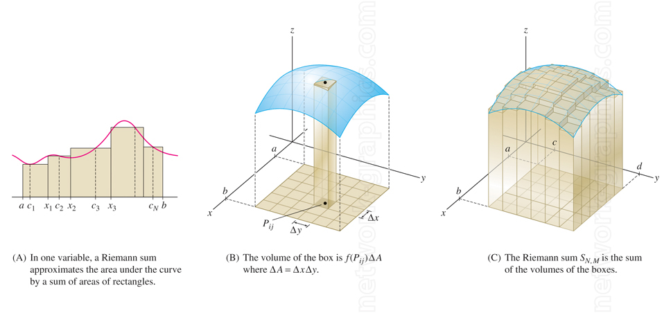
Figure 1: When we were deriving an expression for the definite integral in terms of the Riemann sum, we first approximated the area underneath \(f(x)\) by summing the areas of many very skinny rectangles as illustrated in (A). To define a double integral in terms of a Riemann sum, we first approximate the volume underneath a surface by summing the volumes of many very skinny columns as depicted in (C). The width and depth of each column is given by \(Δx\) and \(Δy\) and the height of each rectangle is given by the surface \(f(x,y)\) as shown in (B).
Let \(f(x,y)\) be any arbitrary function that is smooth and continuous as illustrated in Figure 1(b) and Figure 2. This derivation will be almost identical to the derivation of \(\int{f(x)dx}\) except that we must take the infinite sum of infinitely many infinitesimally skinny columns, not rectangles. How do we construct a very skinny column? As you can see in Figure 2, I have subdivided the interval \(x_n-x_1\) on the \(x\)-axis an \(n\) number of times and the interval \(y_m-y_1\) on the \(y\)-axis an \(m\) number of times. To construct a very skinny volume element \(ΔV\) at the coordinate \((1,1)\), we can take the product
$$ΔV_{1,1}=f(x_1,y_1)Δx_1Δy_1,$$
where \(Δx_1=x_2-x_1\) is the width of the column, \(Δy=y_2-y_1\) is the depth, and \(f(x_1,y_1)\) is the height of the column. To find the volume \(ΔV_{2,2}\) of the column located at the coordinate point \((2,2)\) (see Figure 2), we just need to take the product
$$ΔV_{2,2}=f(x_2,y_2)Δx_2Δy_2,$$
where \(Δx_2=x_3-x_2\) is the width of the column, \(Δy_2=y_3-y_2\) is the depth, and \(f(x_3,y_1)\) is the column's height. But suppose that we wanted to represent the volume of any column underneath \(f(x,y)\); how would we do that? We'll let \(x_i\) be any arbitrary \(x\)-value along the interval \(x_n-x_1\) such that \(i=1,...,n\) where \(n\) is any integer and we'll also let \(y_j\) be any arbitrary \(y\)-value along the interval \(y_m-y_1\) such that \(j=1,...,m\). The volume \(ΔV_{i,j}\) of any column located at some arbitrary coordinate value \((x_i,y_j)\) is given by
$$ΔV_{i,j}=f(x_i,y_j)Δx_iΔy_j.$$
Figure 2: The volume underneath the surface \(f(x,y)\) can be approximated by summing the volumes of an \(nm\) number of columns underneath the surface. As these columns become infinitesimally skinny and as the number \(nm\) of them approaches infinity, this sum gives the exact volume underneath the surface \(f(x,y)\).
To approximate the volume underneath the surface \(f(x,y)\), let's take the Riemann sum of every volume element \(ΔV_{i,j}\) to get
$$\text{Volume underneath f(x,y)}≈\sum_{i,j}^{n,m}f(x_i,y_j)Δx_iΔy_j.$$
Let me take a moment to explain the summation notation for a sum with two indices (in this example, \(i\) and \(j\)). The way that this sum works is by first taking the sum from \(i=1\) to \(i=n\) (while keeping \(j\) a constant at \(j=1\)) to get
$$f(x_1,y_1)Δx_1Δy_1+...+f(x_n,y_1)Δx_nΔy_1.$$
This sum approximates the volume underneath the "edge" of the surface as illustrated in Figure 3. To estimate the volume underneath the adjacent portion of the surface (the highlighted portion represented by \(R_2\)), we need to find the total volume of the adjacent row of columns underneath \(R_2\). This is accomplished by taking the sum from \(i=1\) to \(i=n\) (keeping \(j=2\)) to get
$$f(x_1,y_2)Δx_1Δy_2+...+f(x_n,y_2)Δx_nΔy_2.$$
The expression above approximates the volume underneath the region of the surface designated by \(R_2\). Of course, to approximate the volume underneath both \(R_1\) and \(R_2\) we must add both expressions together to get
$$f(x_1,y_1)Δx_1Δy_1+...+f(x_n,y_1)Δx_nΔy_1.$$
$$+f(x_1,y_2)Δx_1Δy_2+...+f(x_n,y_2)Δx_nΔy_2.$$
The expression approximating the volume underneath \(R_1\), \(R_2\), and \(R_3\) is given by
$$f(x_1,y_1)Δx_1Δy_1+...+f(x_n,y_1)Δx_nΔy_1.$$
$$+f(x_1,y_2)Δx_1Δy_2+...+f(x_n,y_2)Δx_nΔy_2.$$
$$+f(x_1,y_3)Δx_1Δy_3+...+f(x_n,y_3)Δx_nΔy_3.$$
And so on. To approximate the volume underneath the entire surface, we just take the sum
$$f(x_1,y_1)Δx_1Δy_1+...+f(x_n,y_1)Δx_nΔy_1$$
$$+f(x_1,y_2)Δx_1Δy_2+...+f(x_n,y_2)Δx_nΔy_2$$
$$+...+f(x_1,y_m)Δx_1Δy_m+...+f(x_n,y_m)Δx_nΔy_m.$$
The expression, \(\sum_{i,j}^{n,m}f(x_i,y_j)Δx_iΔy_j\), is just a short-hand way of representing the equation above—that's all it is. Also, we can rewrite this sum as
$$\sum_{i,j}^{n,m}f(x_i,y_j)Δx_iΔy_j=\sum_{j=1}^m(\sum_{i=1}^nf(x_i,y_j)Δx_iΔy_j).$$
The equation on the right-hand side is basically the same thing as the one on the left-hand side except the order of addition of each volume element is changed. To evaluate the sum on the right-hand side, we first evaluate the sum
$$\sum_{i=1}^nf(x_i,y_j)Δx_iΔy_j=f(x_1,y_j)Δx_1Δy_j+...+f(x_n,y_j)Δx_nΔy_j.$$
Then, we just take a sum of this result from \(j=1\) to \(j=m\) to get
$$\sum_{j=1}^m\sum_{i=1}^nf(x_i,y_j)Δx_iΔy_j=f(x_1,y_1)Δx_1Δy_1+...+f(x_n,y_1)Δx_nΔy_1$$
$$+f(x_1,y_2)Δx_1Δy_2+...+f(x_n,y_2)Δx_nΔy_2+...+f(x_1,y_m)Δx_1Δy_m+...+f(x_n,y_m)Δx_nΔy_m.$$
Although the equation above is pretty ugly to look at, if we change the order of the sum of each of the terms, we'll end up with the same sum as \(\sum_{i,j}^{n,m}f(x_i,y_j)Δx_iΔy_j\). Both sums are totally equivalent. Recall that to get the exact area underneath an arbitrary curve \(f(x)\), we had to let the width of each rectangle approach zero and the sum become infinite; analogously, in this situation, we must let the width and depth of each column approach zero (that way, they are infinitesimally skinny) and the sum become infinite (meaning, we'll be taking the sum of the volumes of infinitely many columns) to find the exact volume underneath the surface \(f(x,y)\). Doing this, we have
$$\lim_{Δx_i→0,Δy_j→0}\sum_{j=1}^m\sum_{i=1}^nf(x_i,y_j)Δx_iΔy_j.$$
As the number of columns becomes infinite, the variables \(x_i\) and \(y_j\) become continuous (\(x_i→x\) and \(y_i→y\)), the widths and depths of each column becomes infinitesimal (\(Δx→dx\) and \(Δy→dy\)), and the two finite sums turn into infinite sums (\(\sum_{i=1}^n→∫\) and \(\sum_{j=1}^m→∫\)). Thus, the equation above becomes\(^1\)
$$∫∫f(x,y)dxdy≡\lim_{Δx_i→0,Δy_j→0}\sum_{j=1}^m\sum_{i=1}^nf(x_i,y_i)Δx_iΔy_j.$$
This article is licensed under a CC BY-NC-SA 4.0 license.
Notes
1. I have also inserted the symbol "\(≡\)" to represent the fact that the double integral is defined as the quantity on the right-hand side of the equation below.