In this lesson, we'll use Guass's law to find the electric field generated by a parallel-plate capacitor. A parallel-plate capacitor is a capacitor whose conductors are plates which are aligned parallel to one another and seperated by some kind of insulative material. For the purposes of this derivation, we'll assume that the two conductors are separated by a vacuum. We'll begin by first using Guass's law to derive the electric field produced by a single charged plate. (After that, we'll have found the electric field \(\vec{E}_1\) for Plate 1 and the electric field \(\vec{E}_2\) for plate 2. Finding the total electric field \(\vec{E}\) produced by both plates will then simply be just a matter of taking the sum \(\vec{E}_1+\vec{E}_2\) - but we'll cover this a little later on in the derivation.)

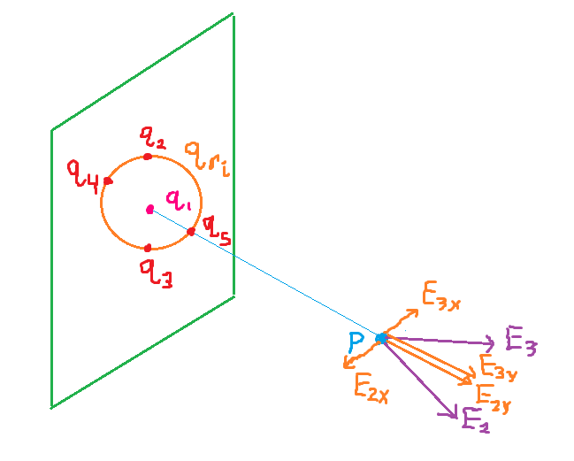
Figure 1.
As we learned in the lessons on Gauss's law, we must choose an imaginary closed surface (called a Guassian surface) which simplifies the integral \(∯\vec{E}·d\vec{A}\) to \(E∯dA=E(\text{surface area})\). Like in many other problems involving Guass's law, we'll use symetry arguments to simplify that integral. Let \(P\) be any point in the space surrounding the charged plate. The charge \(q_1\) illustrated in Figure 1 will obviously (according to the equation \(\vec{E}=k\vec{q_1}{r^2}\hat{r}\)) generate an electric field which only has an x-component. (This electric field will either point in the positive or negative x-direction depending on whether or not \(q_1\) is positively or negatively charged.) The electric field generated by the ring of charge \(q_{ring 1}\) will also only have an x-component. To understand why, let \(q_i\) and \(q_j\) be any pair of two point charges on opposite sides of the ring of charge. (They could, for example, be the two point charges \(q_2\) and \(q_3\) or the two point charges \(q_4\) and \(q_5\).) The electric field \(\vec{E}_i\) generated by \(q_i\) is \(k\vec{q_i}{r^2}\hat{r}_i\) and the electric field generated by \(q_j\) is \(\vec{E}_j=k\frac{q_j}{r^2}\hat{r}_j\). Since the chared plate is being modeled as being composed of myriad equally charged particles and since \(q_i\) and \(q_j\) are equally far away from the point \(P\), both charged particles generate an equally strong electric field at the point \(P\) (\(E_i=E_j\)). But notice how the directions of \(\vec{E}_i\) and \(\vec{E}_j\) are different in such a way that when they are added, there x-components cancel. To find the total electric field produced by the ring of charge, we must add up the electric fields due to every p[air of charges comprising the ring and, doing so, the x-component of the electric field cancels for every pair of charges. Thus, the entire ring of charge produces an electric field which points only along the x-axis. This cancellation also occurs for every other ring of charge illustrated in Figure 1. This allows us to approximate that the electric field produced by the charged plate is entirely along the x-axis.

Figure 2
Sorry if that discussion seemed rather long-winded, but know this fact allows us to appropriately choose our Guassian surface. We'll choose our Guassian surface to be the cylinder illustrated in Figure 2. The total electric flux \(\phi_E\) through the entire cylinder is the same as the sum of the electric fluxes through surfaces \(A\) and \(C\) on each end of the cylinder and through surface \(B\) making up the other part of the cylinder as illustrated in Figure 2. In other words,
$$\phi_E=\phi_{E,A}+\phi_{E,B}+\phi_{E,C}.\tag{1}$$
You'll see that Equation (1) will make life much easier. Recall from previous lessons on Guass's law that the vector \(d\vec{A}\) is, by definition, always pointing in an "outward direction" that is normal to the surface. For simplicity, I have illustrated the vector field \(d\vec{A}\) along the Guassian cylinder in Figure 3. I have also illustrated the vector field \(\vec{E}\) in Figure 4, and both vector fields \(d\vec{A}\) and \(\vec{E}\) in Figure 5. Since the vectors \(\vec{E}\) and \(d\vec{E}\) are perpendicular to each other at each point along the surface \(B\), the dot product (the dot product in the integral \(∯_B\vec{E}·d\vec{A}\)) at each point along Surface B simplifies to \(\vec{E}·d\vec{A}=0\). Thus, \(\phi_{E,B}=0\) and Equation (1) simplifies to

Figure 3
$$\phi_E=\phi_{E,A}+\phi_{E,C}.\tag{2}$$
Let's think back to what we learned in the lesson, Electric Flux, where the idea of electric flux was first introduced. We showed that the electric flux through any curved surface is given by the integral \(∬_S\vec{E}·d\vec{A}\). That's just the definition of electric flux. But we also showed that if the surface isn't curved, then the electric flux is simply just given be \(\vec{E}·Δ\vec{A}\). As you can see in Figures 2 and 3, the ends of a cylinder are flaThus, the electric fluxes through surfaces \(A\) and \(B\) are \(\phi_{E,A}=\vec{E}·Δ\vec{A}\) and \(\phi_{E,B}=\vec{E}·Δ\vec{A}\). Substituting these expressions for \(\phi_{E,A}\) and \(\phi_{E,B}\) into Equation (2), we have
$$\phi_E=\vec{E}·Δ\vec{A}+\vec{E}·Δ\vec{A}.\tag{3}
For the electric flux through each surface, if the charged plate is positively charged then Equation (3) simplifies to
$$\phi_E=EΔA+EΔA=2EΔA,\tag{4}$$
and if they are negatively charged then Equation (3) becomes
$$\phi_E=-EΔA-EΔA=-2EΔA.\tag{5}$$
According to Guass's law, Equations (4) and (5) are equal to
$$2EΔA=\frac{q_{enc}}{ε_0}\tag{6}$$
and
$$-2EΔA=\frac{q_{enc}}{ε_0},\tag{7}$$
respectively, where \(q_{enc}\) is the amount of charge enclosed within the Guassian surface. (Don't make the mistake of confusing \(q_{enc}\) with the charge of the entire plate.) We'll assume that the distribution of charges along the plate is uniform. Thus if \(σ=\frac{q_{enc}}{A}\) is the charge density on the plate, then Equations (6) and (7) become
$$2EΔA=\frac{σA}{ε_0}\tag{8}$$
$$-2EΔA=\frac{σA}{ε_0}.\tag{9}$$
Using algebra, we can find that the magnitude of the electric field for each plate is
$$E=\frac{σ}{2ε_0}\tag{10}$$
and
$$E=-\frac{σ}{2ε_0},\tag{11}$$
where Equations (10) and (11) are the magnitudes of the electric fields of the positively and negatively charged plates, respectively. We already know that the x-components of the electric field cancels due to symmetry, but what does the y-component of the electric field look like? For a positively charged plate, the electric field (the components and direction) are given by
$$\vec{E}_R= \frac{σ}{2ε_0}(+\hat{j})\tag{12}$$
and
$$\vec{E}_L=\frac{σ}{2ε_0}(-\hat{j}),\tag{13}$$
where Equations (12) and (13) are the electric field on the right and left sides of the plate, respectively, as illustrated in Figure #. For a negatively charged plate as in Figure #, the electric fields on the right and left sides are
$$\vec{E}_R= \frac{σ}{2ε_0}(-\hat{j})\tag{12}$$
and
$$\vec{E}_L=\frac{σ}{2ε_0}(+\hat{j}),\tag{13}$$
respectively.
Figure 4
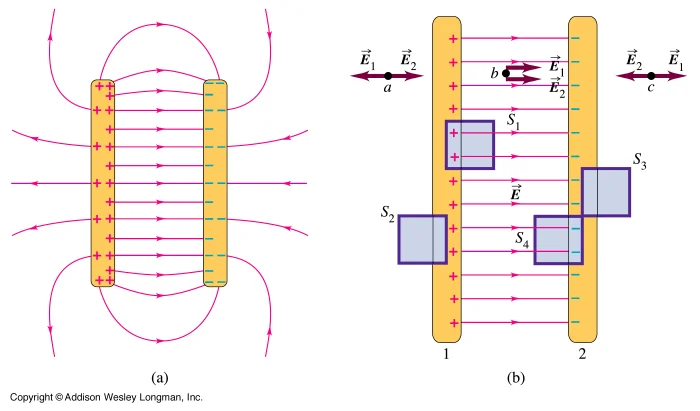
In Figure 4, I have drawn a parallel-plate capacitor. Using Equations (12) and (13), I have drawn the vector field \(\vec{E}_{σ_+}\) produced by the positively charged plate. And using Equations (14) and (15), I have drawn the vector field \(\vec{E}_{σ_-}\) produced by the negatively charged plate. To find the total electricl field produced by both plates (the parallel-plate capacitor), we must take the sum, \(\vec{E}_{σ_+}+\vec{E}_{σ_-}\), of both electric fields. Doing so on the "left" side of the capacitor (see Figure #), we find that the total electric field is
$$\vec{E}=\vec{E}_{σ_+}+\vec{E}_{σ_-}=\frac{σ}{2ε_0}(-\hat{j})+\frac{σ}{2ε_0}(+\hat{j})=0.\tag{16}$$
The electric field produced by the capacitor on the "right" is
$$\vec{E}=\vec{E}_{σ_+}+\vec{E}_{σ_-}=\frac{σ}{2ε_0}(+\hat{j})+\frac{σ}{2ε_0}(-\hat{j})=0.\tag{17}$$
But notice how that in the "middle" (in between the two plates of the capacitor) the electric fields reinforce one another to give a total electric field of
$$\vec{E}=\vec{E}_{σ_+}+\vec{E}_{σ_-}=\frac{σ}{2ε_0}(\hat{j})+\frac{σ}{2ε_0}(\hat{j})=\frac{σ}{ε_0}(\hat{j}).\tag{18}$$
From Equations (16)-(18), we can see that a charged parallel-plate capacitor producesa constant electric field \(\frac{σ}{ε_0}\hat{j}\) in between the plates where the electric field points from the positively charged plate to the negatively charged plate and we can also see that everywhere to the "left" and "right" of the capacitor the electric field is zero. Since the electric field produced in between both plates of the capacitor is a constant, this makes find the voltage \(ΔV\) across the capacitor very simple. The general expression for the voltage between any two points is
$$ΔV_{BA}=\int_B^A\vec{E}·d\vec{l}.$$
Since the electric field in between the capacitor is constant and since the electric force is conservative, we can simplify the expression for the voltage across a parallel-plate capacitor to
$$ΔV_{BA}= \frac{σ}{ε_0}\int_B^Adl=\frac{σ}{ε_0}d,\tag{19}$$
where \(V_B\) is the potential at a point on the positively charged plate, \(V_A\) is the potential on the negatively charged plate, and \(d\) is the separation distance of the two plates.